options(repos = c(CRAN = "https://cloud.r-project.org"))
if (!require("pak")) install.packages("pak")
pkgs = c(
    "sf",
    "tidyverse",
    "tmap",
    "osmextract"
)
pak::pak(pkgs)Prerequisites
1 Course Prerequisites
We assume you are familiar with transport datasets and have basic data analysis skills.
You must have a GitHub account and have saved your username.
We will cover version control concepts in the course.
2 Software Prerequisites
You should bring a laptop with either of the following:
- Option 1: if you’re using a cloud-based development environment:
- A modern web browser (e.g., Chrome, Firefox, Edge).
- A GitHub account (sign up at github.com) and have your username ready.
- Tested out GitHub Codespaces to ensure it works on your machine by opening this link and running the prerequisites code in prerequisites.qmd:
![]()
or, for running the code locally:
- Option 2: A laptop with the necessary software installed, including:
- An IDE such as VS Code (recommended) or RStudio.
- R or Python installed (see below for testing code).
- The
ghcommand-line tool (see cli.github.com for installation and set-up instructions).
3 Recommended Online Courses
To prepare for this course, we recommend watching the following short video:
- Introduction to AI Fluency by Anthropic (Lesson 1, ~5 minutes).
And taking these short but very useful online courses:
- Intro to GitHub (should take less than an hour).
- Communicate using Markdown (should take around 30 minutes or less).
4 Testing your setup
You can test your setup by running the following code in Python or R, either in your local IDE or in GitHub Codespaces. Do so by first creating a new Quarto (.qmd) file, e.g. called test.qmd, and then typing the following into a code chunk with three backticks (located in the top left of your keyboard, just left of the 1 key) to start and end the code chunk and {r} or {python} at the end of the first code chunk to make the code interactive, as follows (update the code as needed):
To run code in .qmd files interactively, ensure your cursor is focused in a code chunk (or you have specific lines of code selected) and then click the “Run Cell” button or (preferably) do it with keyboard shortcuts: press Ctrl+Enter to run the current line or Ctrl+Shift+Enter to run the entire code chunk. See the Quarto documentation at quarto.org/docs/ for more details on how to run code chunks in Quarto.
You should be able to run the code in a GitHub Codespaces with the following link:
![]()
Choose either the Python or R code below, depending on which language you prefer to use.
library(tidyverse)
library(sf)
The next bit optionally downloads lots of data, so you may want to skip it if you’re just testing your setup.
Code
# Centered on Broadway House, London
broadway_house = stplanr::geo_code("Tothill St, London")
# [1] -0.1302077 51.4996820
study_area = st_point(c(-0.13020, 51.4997)) |>
  st_sfc(crs = 4326) |>
  st_transform(27700) |>
  st_buffer(500) |>
  st_transform(4326)
extra_tags = c(
  "maxspeed",
  "lit",
  "cycleway"
)
osm_network = osmextract::oe_get_network(
  place = study_area,
  boundary = study_area,
  boundary_type = "clipsrc",
  extra_tags = extra_tags,
  mode = "driving"
)
sf::write_sf(osm_network, "osm_network.geojson", delete_dsn = TRUE)
u = "https://github.com/itsleeds/ai4transport/raw/main/osm_network.geojson"
osm_network = sf::read_sf(u)If the command above fails, see instructions below:
Your computer cannot access the file osm_network.geojson, perhaps due to a firewall or network issue. You can solve this issue as follows:
Manually download the file from here or if GitHub is blocked, you can access it from OneDrive here.
library(tmap)
# Uncomment the next line to view in interactive window:
# tmap_mode("view")
m = tm_shape(osm_network) +
  tm_lines("maxspeed")
m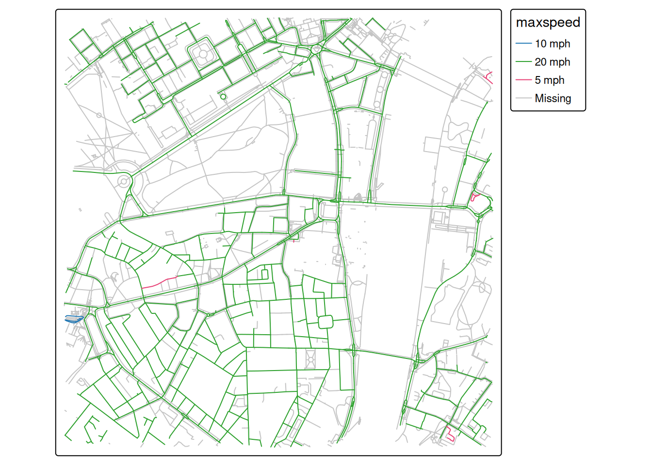
import osmnx as ox
import geopandas as gpd
import matplotlib.pyplot as plt
import shapely

# Import and plot the saved data:
gdf = gpd.read_file("osm_network.geojson")
gdf.explore(column="maxspeed")
# Optional: Download data from OSM:
study_point = shapely.Point(-0.13020, 51.4997)
study_geom = gpd.GeoSeries([study_point], crs=4326)
study_polygon = study_geom.to_crs(epsg=3857).buffer(500).to_crs(epsg=4326).unary_union
study_polygon_gpd = gpd.GeoDataFrame(geometry=[study_polygon], crs="EPSG:4326")
tags = {"highway": True, "maxspeed": True, "lit": True, "cycleway": True}
gdf = ox.features_from_polygon(study_polygon, tags)
gdf = gdf[gdf.geom_type.isin(["LineString", "MultiLineString"])]
gdf = gdf.to_crs(epsg=3857)
gdf.plot(column="maxspeed", figsize=(10, 10), legend=True)
plt.show()If it worked, it should look something like this (from the online development version):
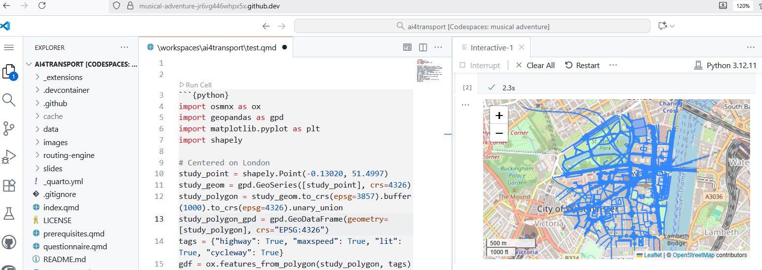
That is the road network surrounding Broadway House in London, where the course will be held in person.
Let us know how you get on and if you have any issues getting set up, either by email, or (preferably) via the Discussion forum on GitHub associated with this course repository.
5 Next Steps
Everyone should complete the Pre-Course Questionnaire before the course begins.
Reuse
Copyright
© 2025 ITS Leeds