9 Raster Data

So far, we have only used Vector data with QGIS; this chapter will introduce raster data.

9.1 What is the difference between raster and vector data.

Vector data is made up of points, lines, and polygons with attributes. This data structure makes it well suited to many GIS purposes. For example, we have already seen that the boundaries of an LSOA can be recorded as a polygon and that each polygon can have attributes like the area name, population etc.

Raster data is very different. It is essentially an image where each pixel has a value. Rasters are always rectangular and have a fixed resolution (so they become pixilated as you zoom in). A common use of raster data is satellite and aerial photography. These images are made from three overlapping rasters (often called a raster stack or raster brick). The three rasters represent the Red, Blue, Green colour bands which together make up a full-colour image. Raster can have more than three bands; for example, they may be used to represent changes over time or colours beyond human perception such as infra-red or ultraviolet.

9.2 Download Sample Data

Download the sample raster data from here:

https://github.com/ITSLeeds/QGIS-intro/releases/download/0.01/leeds_cir_compress.tif

9.3 Adding raster data to the map

Adding raster data to QGIS is done using the same data manager as vector data, except you must use the raster tab. You will notice that the raster contains an aerial photograph of Leeds, except the colours, appear to be wrong.

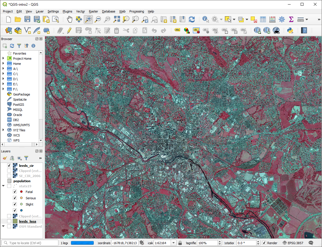
Figure 9.1: The sample raster data added to the map

The colour difference is due to this raster being a colour infrared image. Rather than the usual Red, Green, Blue bands this image has Near Infrared (NI), Red, Green.

9.4 Normalized difference vegetation index

You may have noticed that the trees and grass in the raster appear bright red, but most other features appear grey. We shall use the raster to calculate the Normalized difference vegetation index (NDVI) a measure of how much vegetation is within each raster cell.

Within the “Raster” menu select “Raster Calculator” the formula for calculating the NVDI is:

\[\frac{NI - Red}{NI + Red}\]

Enter the formula into the raster calculator notice the use of @ to designate the different bands of the raster layer. Remember to specify where you want the results to be saved.

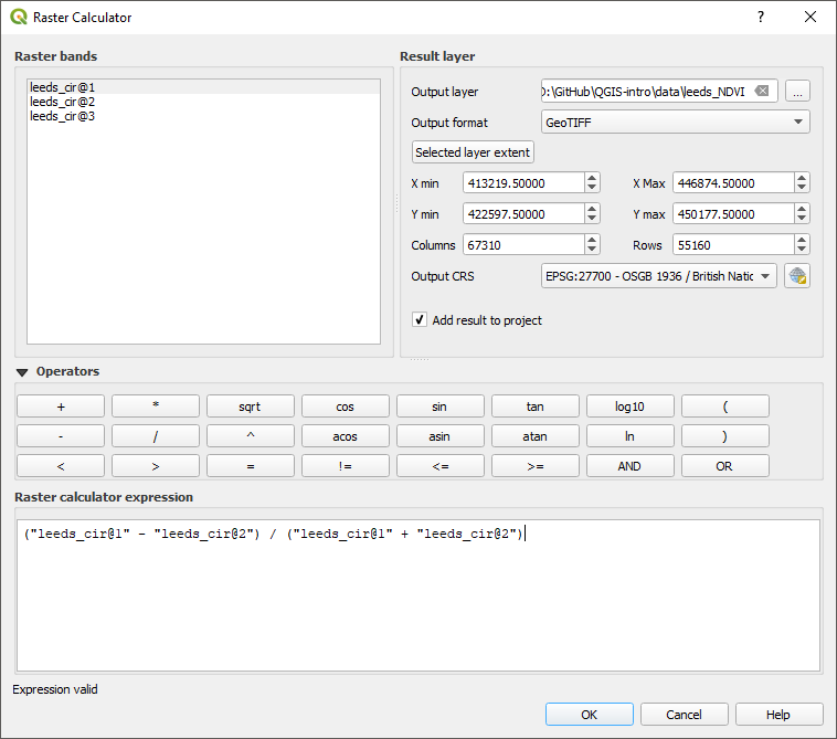
Figure 9.2: The raster calcualtor with the NDVI formula

Once the raster calculator is complete, you should have a new raster layer. It will be in greyscale with values between -1 (least vegetated) and 1 most vegetated. You can adjust the symbology to make the vegetated areas clearer. In the figure, three colours are defined 0 (white), 0.2 (light green), 1 (dark green). These colours approximately make trees dark green, grass light green, and all non-vegetation white.

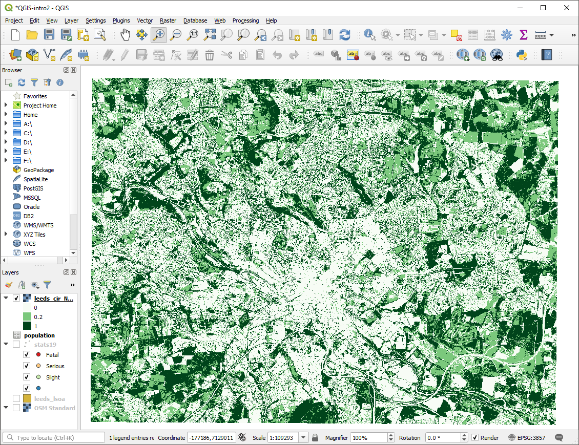
Figure 9.3: The NDVI raster with a psudo-colour scheme applied

9.5 Linking Raster and vector data

Finally, we will link the NDVI raster back to the LSOA boundaries so that we can have an average vegetation score for each LSOA.

In the processing menu select “toolbox”, this opens the processing toolbox panel on the right side. Use the search bar to find the “zonal statistics” tool.

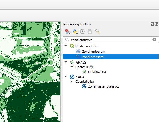
Figure 9.4: The Zonal Statistics tool in the processing toolbox

Complete the form to get statistics from the NDVI raster for each LSOA. When specifying the statistics to calculate select the mean.

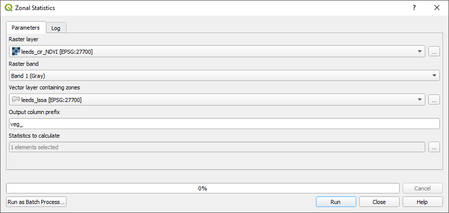
Figure 9.5: The Zonal Statistics tool

Zonal statistics may take several minutes to run. Once completed, the mean NDVI value will be appended to the attribute table of the LSOA polygons.

Adjust the symbology of your LSOA layer to reflect the NDVI scores.

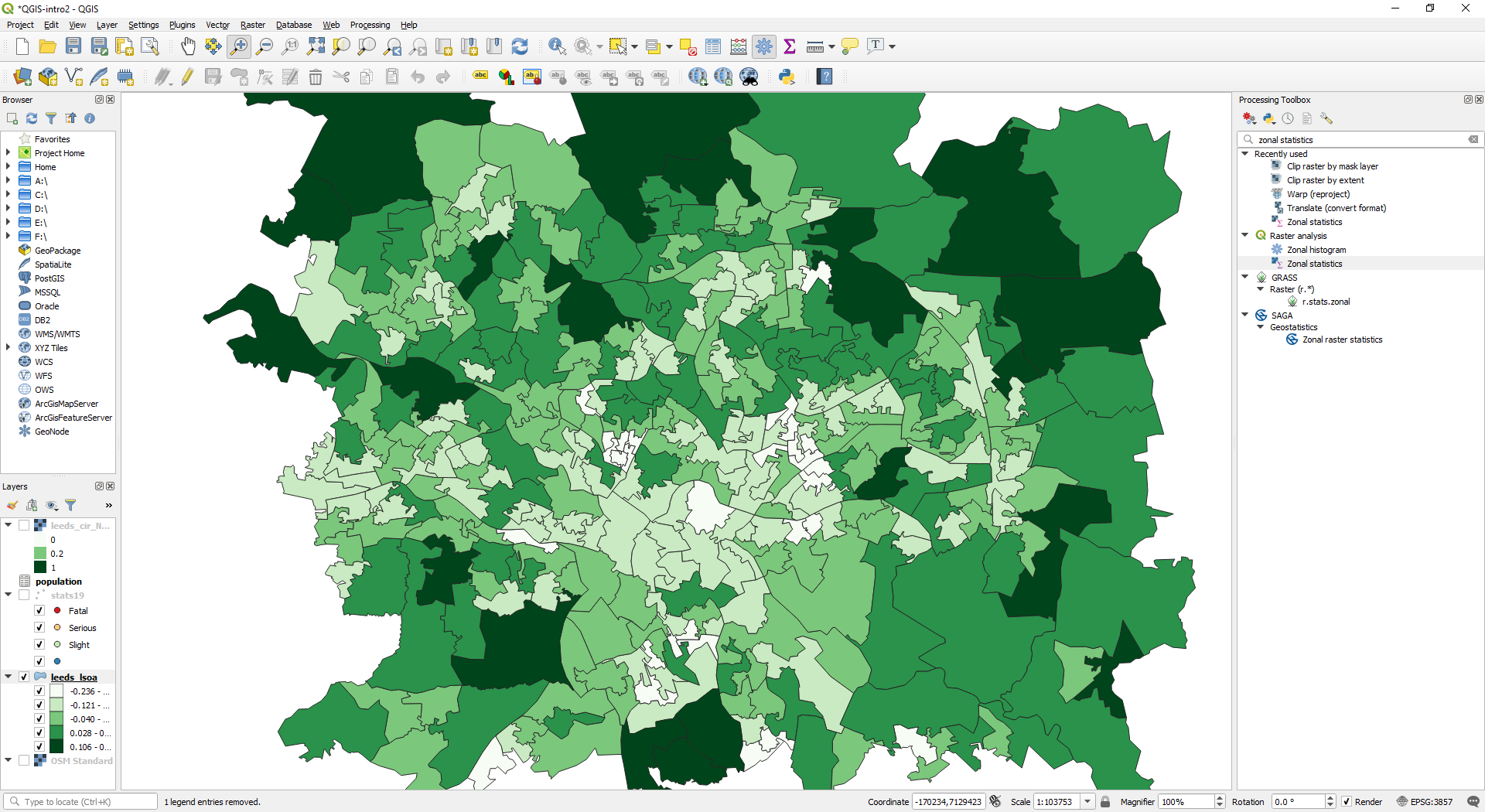
Figure 9.6: LSOA areas with average NDVI scores

9.6 Summary

This chapter has introduced raster data, the raster calculator, and zonal statistics.

Bonus Exercises

Consider how you could use the NDVI values to measure access to green spaces. How might you exclude small areas of green space such as gardens, but include large areas such as parks?