8 Processing vector data

We saw in Chapter 4 how to style and select features of interest from layers loaded into QGIS. In this section, we will learn how to process data. That means creating new data from existing data.

8.1 Reprojecting Data

Two of the three geographic datasets loaded in Chapter 3 have different coordinate systems. This can make it challenging to make connections between the datasets. So we will reproject the stats19 data to the British National Grid.

In the vector, menu select Data management Tools, Reproject Layer.

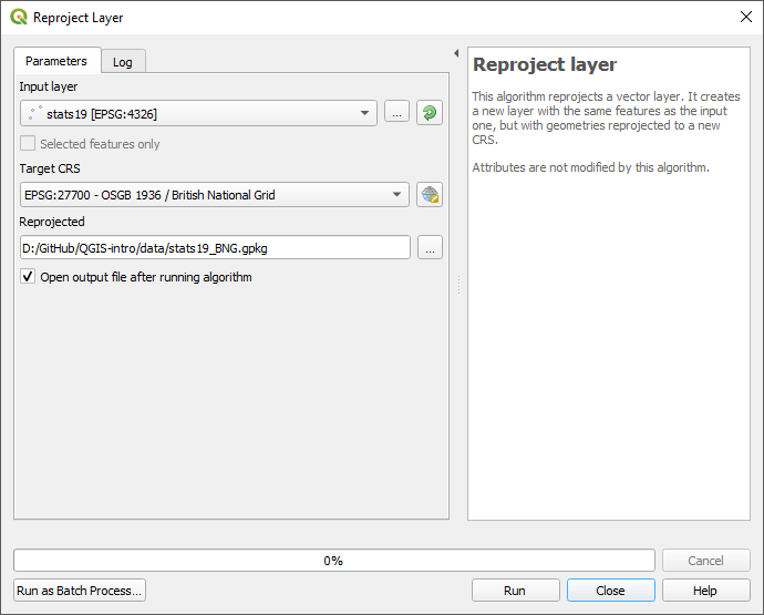
Figure 8.1: Reproject Menu

Then select the British National Grid as the target CRS. If it is not listed in the drop-down menu, then use the button to the right to open the Coordinate Reference System menu. You can use the search box to search for a CRS by name or its EPSG code.

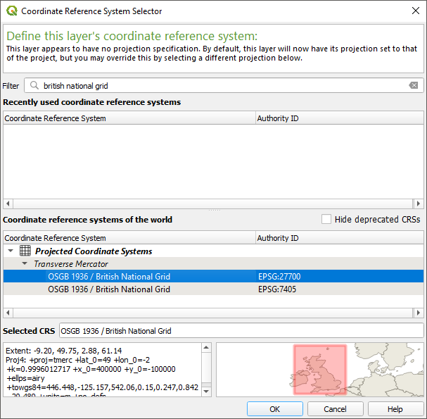
Figure 8.2: Reproject Menu Coordinate Reference System

8.2 Joining Data

Joining data allows you to link two separate datasets together by something they have in common. There are two types of join. Attribute joins (often just called joins) link two datasets by a common attribute such as an ID number. Spatial joins link datasets by a shared location.

In this next section, we will use a series of joins to find the area of Leeds with the highest rate of road collisions.

8.2.1 Attribute Joins

We will join the population data onto the LSOA boundaries.

Find “leeds_lsoa” in the Layers panel and right-click to bring up the context menu.

Click on Properties

Select Joins from the options on the left.

Click the green + button to open the Add Vector Join window.

Select the following options:

Join layer: population

Join field: area

Target field: lsoa11cd

Click OK,

Click OK again

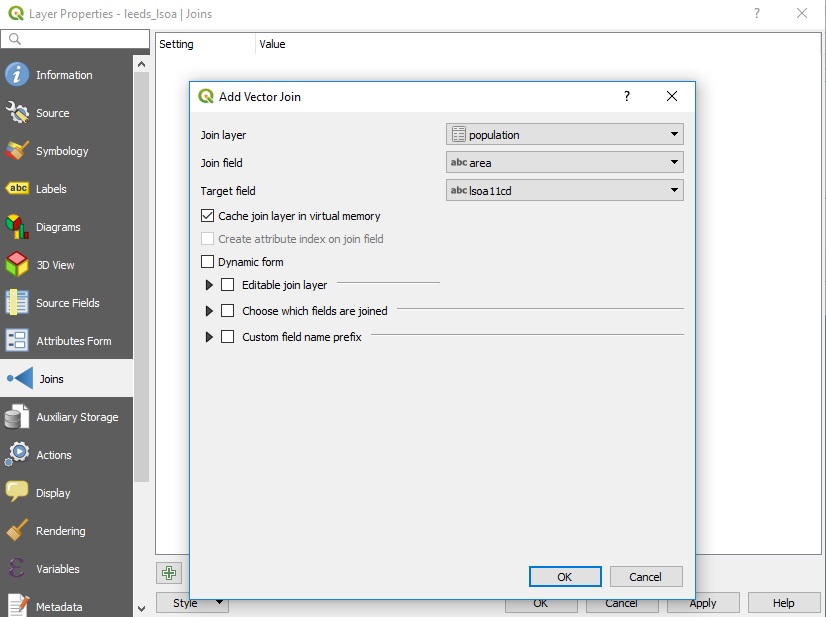
Figure 8.3: The Add Vector Join window

Use the “Identify features” tool to see that each LSOA now has a population value.

8.2.2 Spatial Joins

We will assign an LSOA ID number to each road collision by doing a spatial join.
In the Vector Menu, select Data Management Tools, Select Attributes by location, as shown in 8.4.

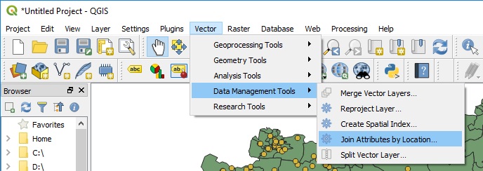
Figure 8.4: Join Attributes by Location

For the Input Layer select “stats19” and for the output later select “leeds_lsoa”. For join type select “Create separate feature of each located feature”. Then click “Run in Background”, as shown in 8.5.

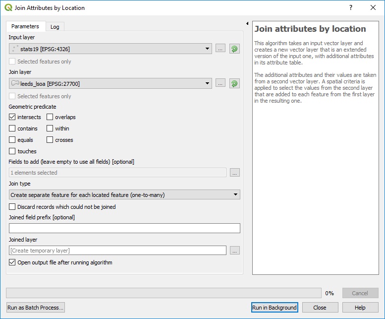
Figure 8.5: Join Attributes by Location Window

Once the process has completed a new layer will have been added to the map called “joined Layer” you can use the “Identify Features” tool to see that each point in the stas19 data now has the new field lsoa11cd containing the LSOA id number for each point in the stats19 data. Manually check a few random points using the “Identify Features” tool to ensure the process has worked correctly.

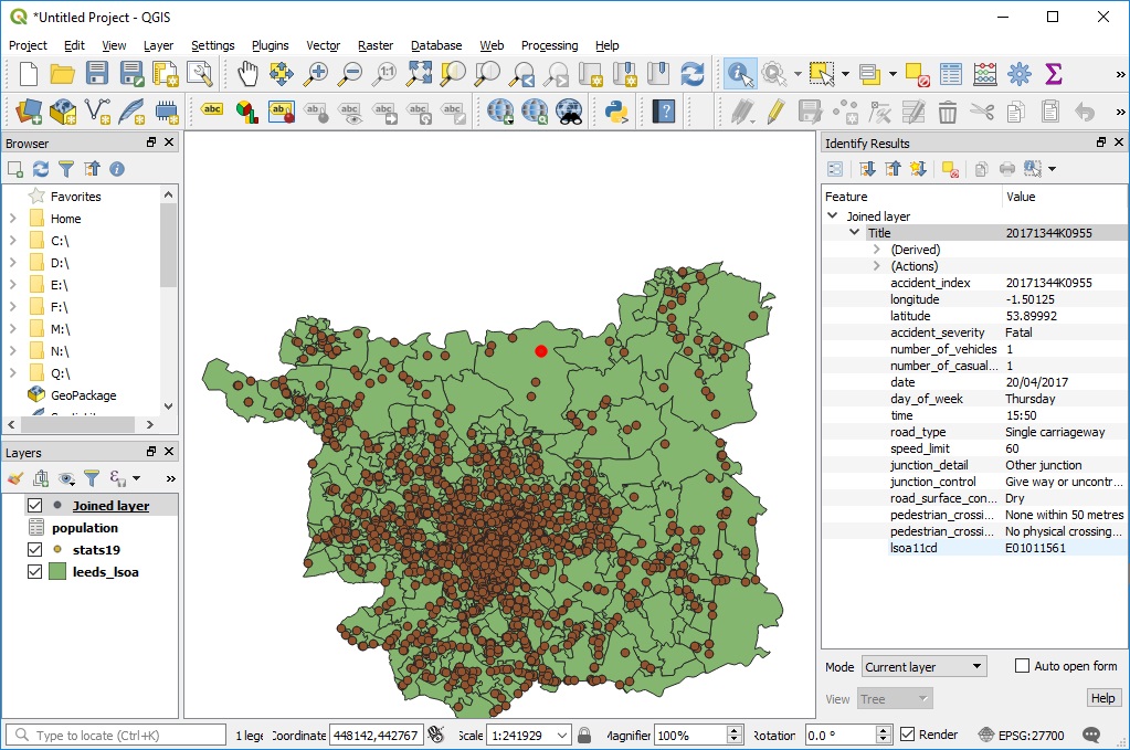
Figure 8.6: Join Results

8.3 Points in Polygons

The final step for this chapter will be to count the number of road crash casualties in each LSOA.

In the Vector Menu, select Analysis Tools, Count Points in Polygons.

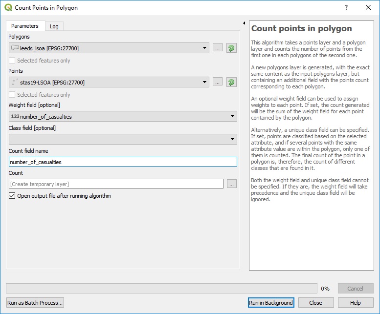
Figure 8.7: Points in Polygons Tool

For the Polygons choose your LSOA areas and the points the stats19 data. USe the number of casualties as a weighting field, and give the “count field name” an appropriate name.

A new layer will be created with the number of casualties for each LSOA. Use symbology to visualise the most dangerous areas of Leeds.

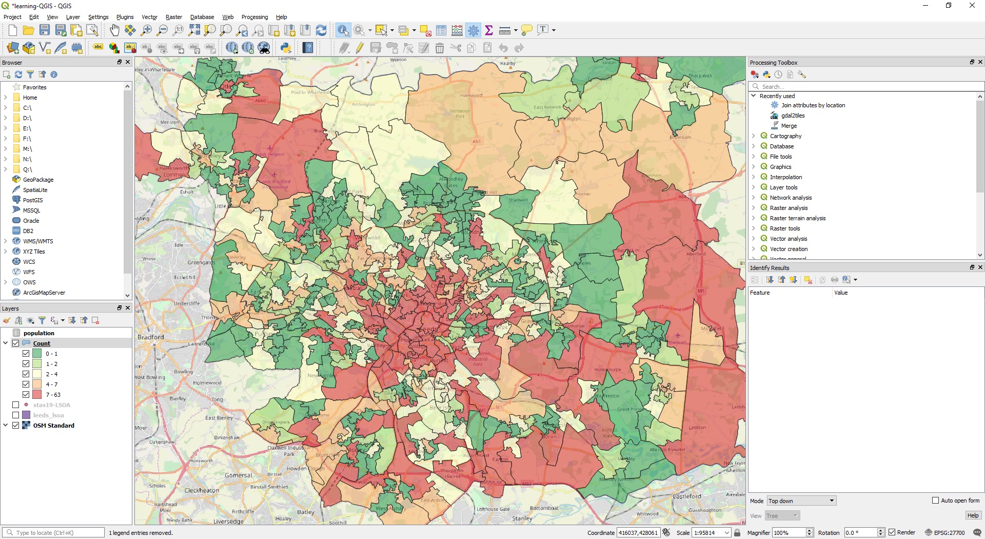
Figure 8.8: Number of road crash casualties in Leeds

8.4 Summary

Before moving onto the next chapter, make sure you have.

1. Reprojected the stats19 data to the British National Grid
2. Done an attribute join of the population data to the LSOA areas
3. Done a spatial join of the LSOA areas to the stats19 points
4. Counted the number of casualties in each LSOA

Bonus Exercises

1. Can you use symbology to show the population of each LSOA?
2. Can you use symbology to indicate the number of casualties in each LSOA?