| date | datetime | Easting | Northing | Severity |
|---|---|---|---|---|
| 2020-09-16 | 2020-09-16 16:16:00 | 541230 | 194939 | Serious |
| 2020-08-27 | 2020-08-27 05:34:00 | 524994 | 292865 | Slight |
| 2020-02-25 | 2020-02-25 17:40:00 | 484904 | 127402 | Slight |
1 Introduction
This book teaches reproducible road safety analysis with R, a popular, free and open-source statistical programming language. It was initially developed for a 2-day course, Introduction to R for Road Safety course. Since then, interest in the topic has grown. The RAC Foundation charity in the UK funded the development of this manual as a free and open-source resource to support their objective of making the roads safer for everyone. The content is based on open-access road crash data from the UK, which is provided by the R package {stats19}. However, the content is designed to be general and should be of use to anyone working with road crash data worldwide, that has (at a minimum) the following variables (see Table 1.1 for an example crash dataset):
- Timestamp
- Location (represented as coordinates as per the table below or address that can be geocoded); and
- Attribute data, such as severity of crash (usually the minimum), and type of vehicles involved (there can be many variables, STATS19 has 50+ attributes, many of which can have more than one value per collision). Additional details are provided in the casualty and vehicle tables.
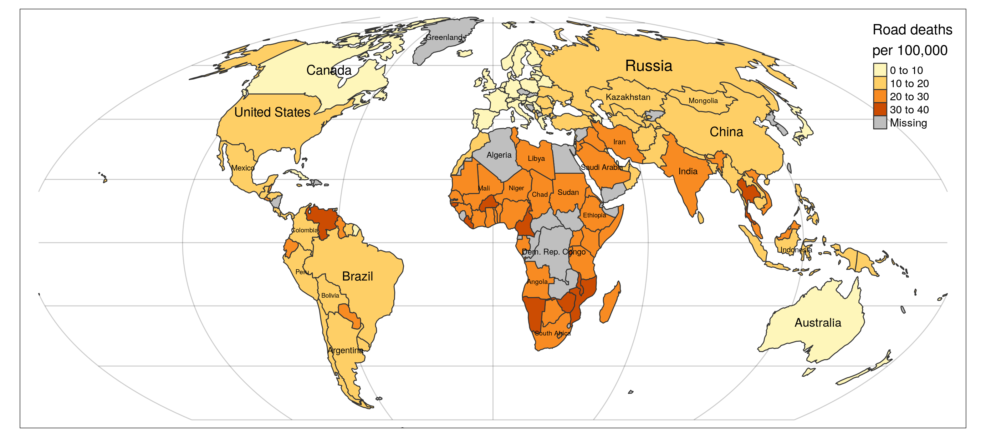
Clearly, work is needed to go from the raw data to evidence that can save lives. Although the datasets used in this guide report road casualty data from Britain, the approach knows no borders: R works equally well in China, India, the USA and Zambia. Road safety is a global issue, that can be considered an epidemic and “the leading cause of death for people aged between 5 and 29 years” worldwide, ahead of hunger, disease and war. The urgency and ubiquity of the ‘road violence’ epidemic is shown in Figure 1.1. Although Britain has relatively safe roads by international standards (with around 3 road traffic deaths per 100,000 people per year, compared with a global average of 17), it still sees over 1000 road deaths each year and unmeasurable costs to families who have lost loved ones and people left with permanent injuries due to poorly designed roads and transport policies.
The guide is practical, meaning that you should reproduce the examples that are provided throughout. As with many practical skills, you learn data science by doing data science.
Before getting stuck in with the practical content, which begins in Chapter 2, the remainder of this chapter:
- introduces the concept of reproducibility and its importance for evidence-based policies;
- explains the choice of R as a ‘tool of the trade’ for road safety research;
- outlines how to install R on your computer or access it through remote servers in the ‘cloud’; and
- explains the structure of the manual, outlines the contents of each section and how they should be used for maximum benefit depending on your level of experience and aims (Section 1.5).
1.1 Reproducibility
Reproducible research can be defined as work that generates results that can be regenerated by others using publicly accessible code. By contrast, findings that cannot be repeated are not reproducible.
Reproducibility is not a binary concept, but a continuum. At one extreme, there is work that does not report the data source, methods or software. At the other end of that continuum, there are findings that can be reproduced in their entirety, including the production of figures and, as is the case with this manual, the manuscript/medium in which results are presented. Reproducibility can be built into every stage of quantitative research, as shown in Table 1.2.
re = readr::read_csv("reproducibility.csv")
knitr::kable(re)
rm(re)| Research component | Requirement |
|---|---|
| Data | Datasets used are available. |
| Methods | Computer code underlying figures, tables, etc are available. Software to execute that code is available. |
| Documentation | Documentation of the computer code, software environment, and methods for others to repeat and build on the analysis. |
| Distribution | Standard methods of distribution are used for others to access the software, data, and documentation. |
The importance of reproducibility in scientific research should be obvious: if findings cannot be repeated, this casts doubt on the validity and truth of the conclusions drawn from them. Reproducibility is vital for falsifiability, a cornerstone of science.
In applied policy-relevant research areas, such as road safety research, reproducibility is equally important: policy makers and the public want to have confidence that the evidence underlying key decisions is reliable. Policies based on results that nobody can reproduce are harder to defend than policies that have a clear evidence base open for others to repeat, including members of the public and educators. In transport planning, open and reproducible methods support more transparent and democratically accountable interventions. Reproducibility leads to solid science, which is conducive to effective policies. In the context of road safety research, this means that reproducibility can save lives.
1.2 What is R?
R is an open-source programming language first developed by award-winning academic statisticians Dr Ross Ihaka and Professor Robert Gentleman. Since its first release in 1995 and the release of version 1.0.0 in 2000, R has seen rapid uptake. As of September 2020, R was ranked as the 9th most used programming language on the TIOBE Index, ahead of other languages for data processing, such as SQL and MATLAB, and behind general-purpose languages such as C, Java and Python.
An important feature of R is that it was designed for data processing and statistical analysis. This means that you can undertake many aspects of road safety research using the core language. R is widely acknowledged to outperform other open languages for data science, such as Julia, Python and Scala, in terms of data visualisation and deployment of web applications for presenting data via the R package shiny. Furthermore, recently developed packages {tidyverse} and {sf}, provide a unified and user-friendly system for working with attribute-rich and geographic datasets. Because road crash data is commonly attribute-rich and geographic, we will be using these packages in subsequent sections.
1.3 Why R for road safety research?
R is an outstanding language for reproducible research. It is accessible with no licensing restrictions and easy installation procedures on a wide range of computers, including most versions of Windows, Mac and Linux operating systems. Furthermore, R is highly extensible. With 2.2607^{4} packages available as of 2025-09-02, many of which are developed by professional statisticians and domain experts, R provides access to a wide array of statistical, computational and visualisation techniques. Many packages, such as {markdown} and {reprex}, were designed to support more reproducible research.
From a road safety perspective, R is well suited to handling data structures used in road safety research. R excels at the processing, analysis, modelling and visualisation of large spatio-temporal and attribute-rich datasets of the type key to road safety research. R is a mature and growing tool for data science, popular in industry, academia and government, so it creates multiple opportunities for collaboration within and between organisations and internationally.
1.4 Prerequisites
You do not need to be a professional programmer, data scientist or computer wizard to use R for road safety research. If you have primarily used graphical user interfaces (GUIs), such as Microsoft Excel, it may take some time to get used to the code-based R approach. However, the command-line interface (CLI) of R is no ‘harder’ than the incessant pointing and clicking demanded by tools such as Excel and web-based GUIs for road safety research. It takes time to adapt to new ways of working, and R has a steep learning curve at the outset. However, persevering can be very rewarding: proficiency with R’s CLI is a future-proof and transferable skill that can yield huge productivity gains. Perhaps the most important prerequisite, therefore, is time and a willingness to try new ways of working.
The good news is that it has never been easier to learn and install R, as highlighted in the {stats19-training-setup} that can be found on the {stats19} package website at docs.ropensci.org/stats19.
It is important to have an up-to-date version of R installed before proceeding to the practical sections of this manual. Note that, like any actively developed software, R is evolving so it is worth updating or re-installing R/RStudio every year or so and updating your R packages every month or so to ensure you have the latest software.
1.5 Installing R and RStudio
To complete the exercises in this guide, you will need to install:
- R from cran.r-project.org
- RStudio from rstudio.com
- R packages, by opening RStudio and typing
install.packages("stats19")in the console to install thestats19package, for example (see Chapter 4 for details)
We recommend using at least the latest stable release of R (4.0.3 at the time of writing in 2020). If you’re running on macOS or Linux, you may need to install additional dependencies, as documented in blog posts and documentation pages such as Installation of R 4.0 on Ubuntu 20.04 LTS and tips for spatial packages and the Installing section of the github.com/r-spatial/sf package README page. We recommend running R on a decent computer, with at least 4 GB RAM and ideally 8 GB or more RAM. R is computationally efficient and therefore a fast language for data science but, because of the size of some road safety datasets, we recommend using it on a high-spec laptop or desktop.
1.6 R in the cloud
If you do not have access to a suitable computer on which you can install R, or just want to get up-and-running quickly, you can run R in the cloud.
Various organisations manage RStudio Server instances, but by far the most well-known cloud provider is at cloud.rstudio.com. To run R in the cloud, sign-up to cloud.rstudio.com (or cloud instance of your choice) and access RStudio from the browser.
1.7 Recommended packages
Of the thousands of available packages that are available for road safety research, we will use a handful that are mature, well-tested and well-suited to statistical analysis and visualisation of road casualty data. For the first practical steps, in Chapter 2, all you need is a working version of R and RStudio. In Chapter 4 we will see how to install and use add-on packages such as {stats19}. If you want to be ahead of the game, you can check that you have the necessary packages installed by running the following commands, which install and load the packages that we will use for the course:
1.8 Overview
The rest of the manual is structured as follows.
- Chapter 2 introduces the basics of the R language. While not essential reading for people who already have experience with R or who just want to get stuck in to importing datasets, as per Chapter 5, it is recommended reading even if you already use R. This section introduces key aspects of the R language that may not be needed for basic data analysis tasks, but which will be vital when ‘debugging’ your code (the process you go through to remove bugs/mistakes). It provides a strong foundation for subsequent sections.
- Chapter 3 provides a brief introduction to productive research workflows using RStudio, an advanced integrated development environment for not only writing R code, but also for project management and boosting your productivity with a suite of features that puts Excel to shame.
- Chapter 4 introduces the
{stats19}package and other R packages we will be using in subsequent chapters. - Chapter 5 demonstrates key data processing techniques using
tidyverse. - Chapter 6 teaches key functions for working with timestamps.
- Chapter 7 shows how you can create maps and perform geographic data analysis with road crash data in R.
- Chapter 8 provides an introduction to joining road crash data, with a focus on casualty and accident tables in STATS19 data (introduced in Chapter 4).
- Chapter 9 suggests next steps for road safety researchers looking to take their skills to the next level and provide the strong evidence needed to save lives.