Calculate cycling uptake for UK 'Government Target' scenario

Uptake model that takes distance and hilliness and returns a percentage of people likely to cycle along a desire line. Source: appendix of pct paper, hosted at: www.jtlu.org which states that:

uptake_pct_govtarget(
  distance,
  gradient,
  alpha = -3.959,
  d1 = -0.5963,
  d2 = 1.866,
  d3 = 0.00805,
  h1 = -0.271,
  i1 = 0.009394,
  i2 = -0.05135
)

uptake_pct_govtarget_2020(
  distance,
  gradient,
  alpha = -4.018,
  d1 = -0.6369,
  d2 = 1.988,
  d3 = 0.008775,
  h1 = -0.2555,
  h2 = -0.78,
  i1 = 0.02006,
  i2 = -0.1234
)

uptake_pct_godutch_2020(
  distance,
  gradient,
  alpha = -4.018 + 2.55,
  d1 = -0.6369 - 0.08036,
  d2 = 1.988,
  d3 = 0.008775,
  h1 = -0.2555,
  h2 = -0.78,
  i1 = 0.02006,
  i2 = -0.1234
)

Arguments

distance	Vector distance numeric values of routes.
gradient	Vector gradient numeric values of routes.
alpha	The intercept
d1	Distance term 1
d2	Distance term 2
d3	Distance term 3
h1	Hilliness term 1
i1	Distance-hilliness interaction term 1
i2	Distance-hilliness interaction term 2
h2	Hilliness term 2

Details

logit (pcycle) = -3.959 +   # alpha
  (-0.5963 * distance) +    # d1
  (1.866 * distancesqrt) +  # d2
  (0.008050 * distancesq) + # d3
  (-0.2710 * gradient) +    # h1
  (0.009394 * distance * gradient) +  # i1
  (-0.05135 * distancesqrt *gradient) # i2

pcycle = exp ([logit (pcycle)]) / (1 + (exp([logit(pcycle)])

uptake_pct_govtarget_2020() and uptake_pct_godutch_2020() approximate the uptake models used in the updated 2020 release of the PCT results.

Examples

distance = 15
gradient = 2
logit_pcycle = -3.959 +   # alpha
  (-0.5963 * distance) +    # d1
  (1.866 * sqrt(distance)) +  # d2
  (0.008050 * distance^2) + # d3
  (-0.2710 * gradient) +    # h1
  (0.009394 * distance * gradient) +  # i1
  (-0.05135 * sqrt(distance) * gradient) # i2
boot::inv.logit(logit_pcycle)
#> [1] 0.0107377
uptake_pct_govtarget(15, 2)
#> [1] 0.0107377
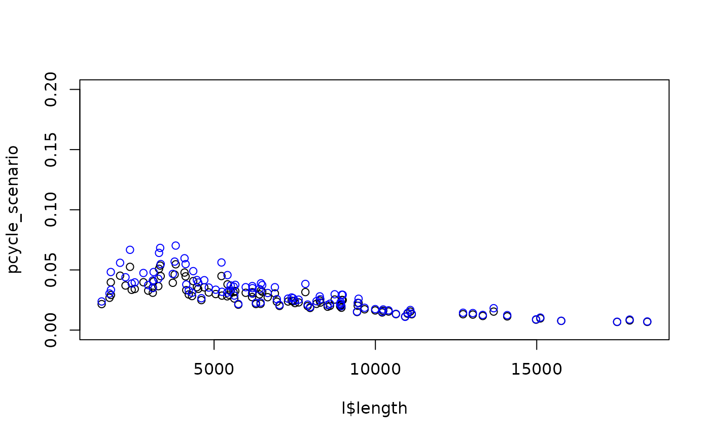
l = routes_fast_leeds
pcycle_scenario = uptake_pct_govtarget(l$length, l$av_incline)
#> Distance assumed in m, switching to km
pcycle_scenario_2020 = uptake_pct_govtarget_2020(l$length, l$av_incline)
#> Distance assumed in m, switching to km
plot(l$length, pcycle_scenario, ylim = c(0, 0.2))
points(l$length, pcycle_scenario_2020, col = "blue")

# compare with published PCT data:
l_pct_2020 = get_pct_lines(region = "isle-of-wight")
# test for another region:
# l_pct_2020 = get_pct_lines(region = "west-yorkshire")
l_pct_2020$rf_avslope_perc[1:5]
#> [1] 0.52 0.30 0.32 0.46 0.49
l_pct_2020$rf_dist_km[1:5]
#> [1] 14.6 11.7 11.3 11.7 12.1
govtarget_slc = uptake_pct_govtarget(
  distance = l_pct_2020$rf_dist_km,
  gradient = l_pct_2020$rf_avslope_perc
) * l_pct_2020$all + l_pct_2020$bicycle
govtarget_slc_2020 = uptake_pct_govtarget_2020(
  distance = l_pct_2020$rf_dist_km,
  gradient = l_pct_2020$rf_avslope_perc
) * l_pct_2020$all + l_pct_2020$bicycle
mean(l_pct_2020$govtarget_slc)
#> [1] 1.233474
mean(govtarget_slc)
#> [1] 1.171526
mean(govtarget_slc_2020)
#> [1] 1.233669
godutch_slc = uptake_pct_godutch(
  distance = l_pct_2020$rf_dist_km,
  gradient = l_pct_2020$rf_avslope_perc
) * l_pct_2020$all + l_pct_2020$bicycle
godutch_slc_2020 = uptake_pct_godutch_2020(
  distance = l_pct_2020$rf_dist_km,
  gradient = l_pct_2020$rf_avslope_perc
) * l_pct_2020$all + l_pct_2020$bicycle
mean(l_pct_2020$dutch_slc)
#> [1] 3.574052
mean(godutch_slc)
#> [1] 3.828446
mean(godutch_slc_2020)
#> [1] 4.191658