Model cycling levels as a function of explanatory variables

model_pcycle_pct_2020(pcycle, distance, gradient, weights)

Arguments

pcycle: The proportion of trips by bike, e.g. 0.1, meaning 10%
distance: Vector distance numeric values of routes in km (switches to km if more than 100).
gradient: Vector gradient numeric values of routes.
weights: The weights used in the model, typically the total number of people per OD pair

Examples

# l = get_pct_lines(region = "isle-of-wight")
# l = get_pct_lines(region = "cambridgeshire")
l = wight_lines_pct
pcycle = l$bicycle / l$all
pcycle_dutch = l$dutch_slc / l$all
m1 = model_pcycle_pct_2020(
  pcycle,
  distance = l$rf_dist_km,
  gradient = l$rf_avslope_perc - 0.78,
  weights = l$all
  )
m2 = model_pcycle_pct_2020(
  pcycle_dutch, distance = l$rf_dist_km,
  gradient = l$rf_avslope_perc - 0.78,
  weights = l$all
)
m3 = model_pcycle_pct_2020(
  pcycle_dutch, distance = l$rf_dist_km,
  gradient = l$rf_avslope_perc - 0.78,
  weights = rep(1, nrow(l))
)
m1
#> 
#> Call:  stats::glm(formula = pcycle ~ distance + sqrt(distance) + I(distance^2) + 
#>     gradient + distance * gradient + sqrt(distance) * gradient, 
#>     family = "quasibinomial", weights = weights)
#> 
#> Coefficients:
#>             (Intercept)                 distance           sqrt(distance)  
#>                -6.79130                 -1.04186                  4.17349  
#>           I(distance^2)                 gradient        distance:gradient  
#>                 0.01768                  0.63445                  0.03433  
#> sqrt(distance):gradient  
#>                -0.48555  
#> 
#> Degrees of Freedom: 136 Total (i.e. Null);  130 Residual
#> Null Deviance:	    657.4 
#> Residual Deviance: 351.3 	AIC: NA
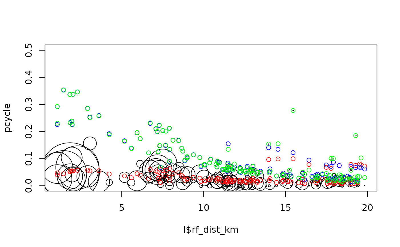
plot(l$rf_dist_km, pcycle, cex = l$all / 100, ylim = c(0, 0.5))
points(l$rf_dist_km, m1$fitted.values, col = "red")
points(l$rf_dist_km, m2$fitted.values, col = "blue")
points(l$rf_dist_km, pcycle_dutch, col = "green")

cor(l$dutch_slc, m2$fitted.values * l$all)^2 # 95% captured
#> [1] 0.9998731
# identical means:
mean(l$dutch_slc)
#> [1] 34.18643
mean(m2$fitted.values * l$all)
#> [1] 34.18643
pct_coefficients_2020 = c(
  alpha = -4.018 + 2.550,
  d1 = -0.6369 -0.08036,
  d2 = 1.988,
  d3 = 0.008775,
  h1 = -0.2555,
  i1 = 0.02006,
  i2 = -0.1234
)
pct_coefficients_2020
#>     alpha        d1        d2        d3        h1        i1        i2 
#> -1.468000 -0.717260  1.988000  0.008775 -0.255500  0.020060 -0.123400 
m2$coef
#>             (Intercept)                distance          sqrt(distance) 
#>             -1.11820425             -0.63433011              1.61587978 
#>           I(distance^2)                gradient       distance:gradient 
#>              0.01071045             -0.43192958             -0.03685552 
#> sqrt(distance):gradient 
#>              0.13203862 
plot(pct_coefficients_2020, m2$coeff)

cor(pct_coefficients_2020, m2$coeff)^2
#> [1] 0.9740929
cor(pct_coefficients_2020, m3$coeff)^2 # explains 95%+ variability in params
#> [1] 0.9653234