PCT / LCWIP Data Ingest & Funding Analysis (2026)

REF 2029 impact case study — England proof-of-concept

1 Overview

This document reports the results of the 2026 re-run of the data-ingest process that collects evidence of the Propensity to Cycle Tool (PCT) and related active-travel planning tools in English Local Cycling and Walking Infrastructure Plans (LCWIPs) and related documents, integrated with official Active Travel Fund (ATF) allocation data.

The 2026 run is a proof-of-concept for England (the first stage before an international roll-out). It improves on previous (~2024) work in four key ways:

1. Distinction between LCWIP reports and related material — each document is classified LCWIP, LCWIP-related, or other, a distinction the previous work did not make.
2. Richer “how PCT was used” detail — explicit scenario usage (Go Dutch, Government Target, E-bike, Go Cambridge), data sources, desire-line usage, and prioritisation-integration flags.
3. Reproducible pipeline — every web page / PDF is downloaded to data-govuk-2026-raw and a .md text extract written to data-govuk-2026-md; structured fields are extracted with a single, unlimited local engine (Ollama gemma4-12b-hermes) so the results are fully reproducible without paid API credits.
4. Integration with Capital & Revenue Funding Data — matching local authority entities to historical ATF funding (2020/21–2024/25) and multi-year future funding allocations (2026–2030) to evaluate how tool adoption aligns with infrastructure investment.

The headline dataset merges the fresh 2026 collection with the existing 94-entry database (LCWIP_database.json), so the release shows how the evidence base has grown.

2 Ingest Methods

• Discovery. Seed URLs came from the existing 94-entry database, supplemented by web searches for 2024–2026 LCWIPs and related active-travel strategies, plus the Transport for the South East (TfSE) Regional Active Travel Strategy and Action Plan (RATSAP) Evidence Base (June 2025), which contains a 64-LCWIP status log for the South East.
• Download. Each candidate URL was fetched and stored as a raw file (data-govuk-2026-raw) with a text/markdown extract (data-govuk-2026-md).
• Extraction. A 21-field schema (schema_2026.json) was applied per document via a local LLM. Outputs are in results/extracted/.
• Aggregation. Extracted records were merged with the 94-entry database by URL/name and written to results.json and a flat results.csv.

3 Corpus Composition

import pandas as pd
df = pd.read_csv("results/results_flat.csv")
print(f"Total merged records: {len(df)}")

Total merged records: 232

print(f"  2026-only: {(df['_source_tag']=='2026').sum()}")

  2026-only: 228

print(f"  from existing 94-DB: {(df['_source_tag']=='existing94').sum()}")

  from existing 94-DB: 4

print()

print("Document type:")

Document type:

print(df['doc_type'].fillna('(unknown)').value_counts())

doc_type
LCWIP            196
other             23
LCWIP-related     10
(unknown)          3
Name: count, dtype: int64

4 PCT Mentions

The central finding for the REF case study is the share of documents that explicitly mention the Propensity to Cycle Tool.

import pandas as pd
df = pd.read_csv("results/results_flat.csv")
pct = df['mentions_pct']
n = pct.notna().sum()
mentioned = (pct == True).sum()
print(f"Documents with a usable mentions_pct flag: {n}")

Documents with a usable mentions_pct flag: 228

print(f"Mention PCT: {mentioned} ({mentioned/n*100:.1f}%)")

Mention PCT: 148 (64.9%)

print(f"Do not mention PCT: {(pct==False).sum()} ({ (pct==False).sum()/n*100:.1f}%)")

Do not mention PCT: 80 (35.1%)

print(f"Unknown (no content / failed download): {pct.isna().sum()}")

Unknown (no content / failed download): 4

4.1 PCT Mentions by Document Type

import pandas as pd
df = pd.read_csv("results/results_flat.csv")
ct = pd.crosstab(df['doc_type'].fillna('unknown'), df['mentions_pct'].fillna('unknown'))
print(ct)

mentions_pct   False  True  unknown
doc_type                           
LCWIP             56   136        4
LCWIP-related      5     5        0
other             17     6        0
unknown            2     1        0

4.2 Change Over Time

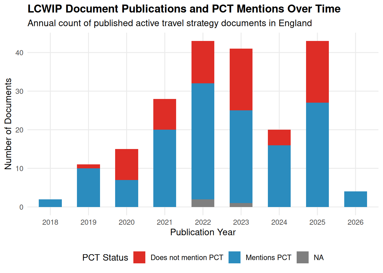
The chart below shows the evolution of LCWIP and active travel document publications over time (2018–2026), categorized by whether the report mentions the Propensity to Cycle Tool.

library(readr)
library(ggplot2)
library(dplyr)

csv_path <- "results/results_flat.csv"
if (!file.exists(csv_path)) csv_path <- "../results/results_flat.csv"

df <- read_csv(csv_path, show_col_types = FALSE) %>%
  mutate(year = readr::parse_number(as.character(date_published))) %>%
  filter(!is.na(year), year >= 2018, year <= 2026)

df_summary <- df %>%
  mutate(pct_label = if_else(mentions_pct, "Mentions PCT", "Does not mention PCT")) %>%
  group_by(year = factor(year), pct_label) %>%
  summarise(count = n(), .groups = "drop")

ggplot(df_summary, aes(x = year, y = count, fill = pct_label)) +
  geom_col(position = "stack", width = 0.6) +
  scale_fill_manual(values = c("Mentions PCT" = "#2b8cbe", "Does not mention PCT" = "#de2d26")) +
  labs(
    title = "LCWIP Document Publications and PCT Mentions Over Time",
    subtitle = "Annual count of published active travel strategy documents in England",
    x = "Publication Year",
    y = "Number of Documents",
    fill = "PCT Status"
  ) +
  theme_minimal(base_size = 12) +
  theme(
    legend.position = "bottom",
    plot.title = element_text(face = "bold"),
    panel.grid.minor = element_blank()
  )

Figure 1: Publication of LCWIP and active-travel planning documents over time by PCT mention status.

5 Scenario Usage

Among documents that mention the PCT, which future scenarios are referenced?

import json, pandas as pd
from collections import Counter
df = pd.read_csv("results/results_flat.csv")
c = Counter()
for _, r in df.iterrows():
    if r.get('mentions_pct') is True or r.get('mentions_pct') == True:
        scs = r.get('pct_scenarios_used')
        if pd.notna(scs):
            if isinstance(scs, str):
                try: scs = json.loads(scs)
                except: pass
            if isinstance(scs, list):
                for s in scs:
                    c[str(s).strip()] += 1
sc = pd.Series(dict(c)).sort_values(ascending=False)
print("Scenario mentions (across PCT-mentioning docs):")

Scenario mentions (across PCT-mentioning docs):

print(sc.to_string())

Go Dutch             79
Government Target    62
E-bike               35
Baseline             24
Go Cambridge          4
Gender Equality       1

6 Geographic Coverage

Coverage against higher-tier authorities in England gives a sense of how much of the country is represented in the corpus.

import pandas as pd
df = pd.read_csv("results/results_flat.csv")
print("Records by region (England):")

Records by region (England):

print(df['region'].fillna('(not stated)').value_counts().to_string())

region
South East                  51
South West                  34
(not stated)                21
East of England             18
North West                  18
West Midlands               16
Yorkshire and the Humber    14
North West England          10
East Midlands               10
North East                   9
South East England           8
West Yorkshire               7
Hertfordshire                3
Surrey                       2
West of England              2
Northwest England            2
D2N2                         2
East                         2
Kent                         1
South West England           1
South Yorkshire              1

print()

print("Records with a combined authority named:")

Records with a combined authority named:

print(df['combined_authority_name'].notna().sum())

43

7 Cost and Network Length

Where stated, LCWIPs propose substantial networks and investment.

import pandas as pd
df = pd.read_csv("results/results_flat.csv")
cost = pd.to_numeric(df['total_cost_pounds'], errors='coerce')
km = pd.to_numeric(df['length_of_network_km'], errors='coerce')
print(f"Documents stating a total cost: {cost.notna().sum()}")

Documents stating a total cost: 46

print(f"Total stated investment (£): {cost.sum():,.0f}")

Total stated investment (£): 23,596,927,576

print(f"Median stated investment (£): {cost.median():,.0f}")

Median stated investment (£): 53,000,000

print(f"Documents stating network length (km): {km.notna().sum()}")

Documents stating network length (km): 33

print(f"Total stated network length (km): {km.sum():,.0f}")

Total stated network length (km): 12,304

8 Illustrative Examples

A sample of LCWIPs that mention the PCT, with how it was used:

import pandas as pd
df = pd.read_csv("results/results_flat.csv")
ex = df[(df['mentions_pct']==True) & (df['doc_type']=='LCWIP')].head(10)
for _, r in ex.iterrows():
    print(f"### {r.get('report_name')} ({r.get('local_authority_name')})")
    print(f"- Date: {r.get('date_published')}")
    print(f"- Scenarios: {r.get('pct_scenarios_used')}")
    print(f"- How used: {str(r.get('how_pct_was_used') or '')[:300]}")
    print()

### Local Cycling and Walking Infrastructure Plan (LCWIP) (Liverpool City Region Combined Authority (LCRCA), in partnership with Halton, Knowsley, Liverpool, Sefton, St Helens, and Wirral councils.[1])
- Date: 2023-09
- Scenarios: ["Government Target", "Go Dutch"]
- How used: The PCT was used to identify potential for cycling growth, analyze existing low-cycling areas with high potential, and compare scenarios to demonstrate the impact of full implementation of the Government’s Cycling and Walking Investment Strategy (CWIS) in the LCR.

### Warwickshire Local Cycling and Walking Infrastructure Plan (Warwickshire County Council)
- Date: February 2024
- Scenarios: nan
- How used: nan

### Banbury Local Cycling and Walking Infrastructure Plan (LCWIP) (Oxfordshire County Council)
- Date: July 2023
- Scenarios: ["Baseline", "Go Dutch", "E-bike"]
- How used: The PCT was used to estimate cycling potential, identify existing and future cycling demand, and inform the prioritisation of the cycle network by highlighting routes with the largest numbers of potential cyclists.

### Local Cycling and Walking Infrastructure Plan – (LCWIP) (Brentwood)
- Date: 2025
- Scenarios: nan
- How used: Referenced in Appendix D (WSP Technical Report) as a primary data source under Stage 2 (Gathering Information) and contrasted against WSPs custom GIS network model which evaluates destinations beyond PCT commute and school trips.

### Cambridgeshire’s Local Cycling and Walking Infrastructure Plan (Cambridgeshire County Council)
- Date: 2022
- Scenarios: nan
- How used: The tool was used to establish the propensity to cycle based on trip distance, identifying that the peak distance for cycling is 2km, with the majority of trips between 1km and 5km. It helped analyze the cycling distance for mapped trips from the 2011 Census data.

### Crawley Local Cycling and Walking Infrastructure Plan (Crawley Borough Council)
- Date: July 2023
- Scenarios: ["Government Target", "Go Dutch"]
- How used: The PCT was used to identify likely route corridors for cycling to work or school, compare them with manually mapped desire lines, and generate estimates of potential cycle rates based on policy targets.

### Carlisle Local Cycling and Walking Infrastructure Plan (LCWIP) 2022 - 2037 (Cumbria County Council)
- Date: March 2022
- Scenarios: nan
- How used: The Propensity to Cycle Tool (PCT) was used as a data source to identify the most popular cycle routes for school and travel-to-work journeys within the district.

### Workington Local Cycling and Walking Infrastructure Plan (LCWIP) 2022 - 2037 (Cumbria County Council)
- Date: June 2022
- Scenarios: nan
- How used: The Propensity to Cycle Tool (PCT) was used as a data source to identify the most popular cycle routes for school and travel to work journeys.

### LOCAL CYCLING AND WALKING INFRASTRUCTURE PLAN Durham City (Durham County Council)
- Date: January 2021
- Scenarios: nan
- How used: The Propensity to Cycle Tool (PCT) was used as one of the key datasets to inform the development of network plans for cycling.

### LOCAL CYCLING AND WALKING INFRASTRUCTURE PLAN Shildon (Blackburn with Darwen Borough Council)
- Date: September 2022
- Scenarios: nan
- How used: PCT-derived cycling demand data (PCTx6) used in route prioritisation scoring criteria.

9 Comparing PCT Evidence with Active Travel Funding

To evaluate the real-world policy and financial impact of the Propensity to Cycle Tool, we link the extracted LCWIP evidence with official UK Government funding datasets from the Active Travel Local Transport Authority Allocations, Departmental Expenditure Limits (RDEL and CDEL), and Active Travel England Capability Ratings 2025.

library(tidyverse)
library(readr)
library(sf)
library(dplyr)
library(jsonlite)
library(stringdist)
library(stringr)
library(DT)

9.1 Data Sources

# 1. Results data from extraction
results_file <- "results/results.csv"
if (!file.exists(results_file)) results_file <- "results/results_flat.csv"
if (!file.exists(results_file)) results_file <- "results_flat.csv"
results <- read_csv(results_file, show_col_types = FALSE)

# 2. LAD and Transport Authority geometry/names from uktransportauthorities
geojson_file <- "data/transport_authorities_2026.geojson"
if (!file.exists(geojson_file)) geojson_file <- "tda/transport_authorities_2026.geojson"
if (!file.exists(geojson_file)) geojson_file <- "transport_authorities_2026.geojson"

if (file.exists(geojson_file)) {
    ltas <- sf::read_sf(geojson_file)
} else {
    ltas <- sf::read_sf("https://raw.githubusercontent.com/itsleeds/uktransportauthorities/refs/heads/main/transport_authorities_2026.geojson")
}

# 3. Historical ATF Allocations (2020/21 - 2024/25)
atf_file <- "data/atf_table_aggregated.csv"
if (!file.exists(atf_file)) atf_file <- "tda/atf_table_aggregated.csv"
if (!file.exists(atf_file)) atf_file <- "scripts/atf_table_aggregated.csv"
if (!file.exists(atf_file)) atf_file <- "atf_table_aggregated.csv"

if (file.exists(atf_file)) {
    atf <- read_csv(atf_file, show_col_types = FALSE)
} else {
    atf <- read_csv("https://raw.githubusercontent.com/itsleeds/uktransportauthorities/refs/heads/main/atf_table_aggregated.csv", show_col_types = FALSE)
}

# 4. Future ATF Multi-Year Allocations (2026 - 2030)
future_file <- "data/lad_active_travel_allocations.csv"
if (!file.exists(future_file)) future_file <- "tda/lad_active_travel_allocations.csv"
if (!file.exists(future_file)) future_file <- "lad_active_travel_allocations.csv"

if (file.exists(future_file)) {
    atf_future <- read_csv(future_file, show_col_types = FALSE)
} else {
    atf_future <- read_csv("https://raw.githubusercontent.com/itsleeds/uktransportauthorities/refs/heads/main/lad_active_travel_allocations.csv", show_col_types = FALSE)
}

9.2 Entity Reconciliation & Name Matching

To ensure accurate joins between LCWIP reports and funding allocations, local authority names are cleaned and matched using Jaro-Winkler string distance with manual alias rules for reconfigured unitary and combined authorities.

# Extract unique authority names from extraction results
results_names <- results |>
    select(local_authority_name, combined_authority_name) |>
    mutate(name = ifelse(
        !is.na(local_authority_name), 
        local_authority_name, 
        combined_authority_name
    )) |>
    distinct(name) |>
    arrange(name) |>
    filter(!is.na(name))

# Extract names from LTAs and unpack JSON lookup
ltas_names <- ltas |>
    st_drop_geometry() |>
    select(name, lad_lookup) |>
    arrange(name) |>
    rename(name_lookup = lad_lookup)

ltas_lookup_names <- ltas_names |>
    mutate(name_lookup = map(
        name_lookup, 
        ~ fromJSON(.x)$lad_name
    )) |>
    select(name, name_lookup) |>
    unnest(name_lookup)

ltas_lookup_names <- bind_rows(
    ltas_lookup_names,
    ltas_lookup_names |>
        distinct(name) |>
        filter(!name %in% ltas_lookup_names$name_lookup) |>
        mutate(name_lookup = name)
)

# Standardise names by stripping council boilerplate
results_names <- results_names |>
    mutate(name_clean = name |>
        str_remove_all("(?i)city") |>
        str_remove_all("(?i)councils") |>
        str_remove_all("(?i)council") |>
        str_remove_all("Borough") |>
        str_remove_all("(?i)district") |>
        str_remove_all("(?i)county") |>
        str_remove_all("(?i)of") |>
        str_remove_all("(?i)the") |>
        str_remove_all("(?i) and") |>
        str_remove_all("(?i)royal") |>
        str_remove_all("(?i)combined authority") |>
        str_remove_all("(?i)metropolitan") |>
        str_remove_all("(?i)(national guidance)") |>
        str_remove_all("(?i)&") |>
        str_remove_all("(?i),") |>
        str_remove_all("(?i)/") |>
        str_squish()
    )

# Add manual aliases for known boundary reconfigurations
manual_aliases_ltas <- tibble(
    name = c(
        "Kent",
        "West Yorkshire Combined Authority",
        "Bournemouth, Christchurch and Poole",
        "West of England Combined Authority",
        "Leicestershire",
        "Norfolk",
        "East Midlands Combined Authority",
        "North East Combined Authority",
        "East Riding of Yorkshire",
        "West Yorkshire Combined Authority",
        "Liverpool City Region Combined Authority",
        "Leicestershire",
        "Lancashire",
        "Leicestershire"
    ),
    name_lookup = c(
        "Faversham Town",
        "West Yorkshire",
        "BCP",
        "Bath North East Somerset Bristol South Gloucestershire North Somerset",
        "Blaby",
        "Broads Authority",
        "Derby Derbyshire Nottingham Nottinghamshire",
        "Durham",
        "Hull",
        "Leeds West Yorkshire",
        "Liverpool Region (LCRCA) in partnership with Halton Knowsley Liverpool Sefton St Helens Wirral",
        "North West Leicestershire",
        "Preston South Ribble Chorley",
        "Rutland"
    )
)

ltas_lookup_names <- bind_rows(ltas_lookup_names, manual_aliases_ltas) |>
    distinct(name, name_lookup, .keep_all = TRUE) |>
    arrange(name, name_lookup)

# String distance fuzzy matching (Jaro-Winkler)
results_names <- results_names |>
    mutate(
        match_index = amatch(
            name_clean,
            ltas_lookup_names$name_lookup,
            method = "jw",
            maxDist = 0.25
        ),
        matched_name = ifelse(!is.na(match_index), ltas_lookup_names$name_lookup[match_index], NA_character_),
        ltas_name = ifelse(!is.na(match_index), ltas_lookup_names$name[match_index], NA_character_)
    )

9.3 ATF Name Harmonisation

# Clean historical ATF table
atf <- atf |> filter(name != "Total")
atf_names <- atf |>
    mutate(name = case_when(
        name == "West Midlands ITA" ~ "West Midlands Combined Authority",
        name == "North East Joint Transport Committee" ~ "North East Combined Authority",
        TRUE ~ name
    ))

# Clean future allocations & aggregate East Midlands Combined County Authority
emca_la_list <- c(
    "Derby", "Derbyshire", "Nottingham", "Nottinghamshire", 
    "Leicester", "Leicestershire", "North East Lincolnshire", 
    "North Lincolnshire", "Lincolnshire", "Rutland"
)

emca_la <- atf_future |>
    filter(name %in% emca_la_list) |>
    summarise(across(where(is.numeric), sum, na.rm = TRUE)) |>
    mutate(
        name = "East Midlands Combined Authority", 
        name_atf = "East Midlands Combined County Authority"
    )

atf_future_names <- atf_future |>
    filter(!name %in% emca_la_list) |>
    bind_rows(emca_la) |>
    distinct(name, .keep_all = TRUE) |>
    arrange(name)

9.4 Integrated Metric Construction

We aggregate document observations, depth-of-use scores, desire-line usage, and total funding amounts:

analysis <- ltas_lookup_names |>
    select(name) |>
    distinct(name) |>
    arrange(name)

results_analysis <- results |>
    left_join(
        results_names |> select(local_authority_name = name, ltas_name),
        by = "local_authority_name"
    )

analysis_data <- analysis |>
    left_join(
        results_analysis |>
            mutate(pct_usage_depth = parse_number(as.character(pct_usage_depth))) |>
            group_by(ltas_name) |>
            summarise(
                n_observations = n(),
                n_mentions_pct = sum(n_mentions_pct, na.rm = TRUE),
                pct_usage_depth_1 = sum(pct_usage_depth == 1, na.rm = TRUE),
                pct_usage_depth_2 = sum(pct_usage_depth == 2, na.rm = TRUE),
                pct_usage_depth_3 = sum(pct_usage_depth == 3, na.rm = TRUE),
                n_pct_desire_lines_used = sum(pct_desire_lines_used, na.rm = TRUE)
            ),
        by = c("name" = "ltas_name")
    ) |>
    left_join(
        atf_names |> select(name, atf20_21, atf21_22, atf22_23, atf23_24, atf24_25),
        by = "name"
    ) |>
    left_join(
        atf_future_names |> select(name, cdel_per_year_4yr, rdel_per_year_3yr, total_over_4yr),
        by = "name"
    ) |>
    mutate(across(
        c(atf20_21, atf21_22, atf22_23, atf23_24, atf24_25, cdel_per_year_4yr, rdel_per_year_3yr, total_over_4yr),
        ~ {
            x <- stringr::str_squish(as.character(.x))
            x[stringr::str_detect(x, stringr::regex("^invalid\\s*number$", ignore_case = TRUE))] <- NA_character_
            readr::parse_number(x)
        }
    ))

funding_5yr_cols <- c("atf20_21", "atf21_22", "atf22_23", "atf23_24", "atf24_25")

analysis_metrics <- analysis_data |>
    mutate(
        n_observations = replace_na(n_observations, 0),
        n_mentions_pct = replace_na(n_mentions_pct, 0),
        n_pct_desire_lines_used = replace_na(n_pct_desire_lines_used, 0),
        pct_usage_depth_1 = replace_na(pct_usage_depth_1, 0),
        pct_usage_depth_2 = replace_na(pct_usage_depth_2, 0),
        pct_usage_depth_3 = replace_na(pct_usage_depth_3, 0),
        n_depth_scored = pct_usage_depth_1 + pct_usage_depth_2 + pct_usage_depth_3,
        depth_score_mean = if_else(
            n_depth_scored > 0,
            (1 * pct_usage_depth_1 + 2 * pct_usage_depth_2 + 3 * pct_usage_depth_3) / n_depth_scored,
            NA_real_
        ),
        total_over_5yr = if_else(
            rowSums(!is.na(across(all_of(funding_5yr_cols)))) > 0,
            rowSums(across(all_of(funding_5yr_cols)), na.rm = TRUE),
            NA_real_
        ),
        pct_mention_rate = if_else(n_observations > 0, n_mentions_pct / n_observations, NA_real_),
        desire_lines_rate = if_else(n_observations > 0, n_pct_desire_lines_used / n_observations, NA_real_)
    )

9.5 Ranked Metrics Table

The table below displays the resulting dataset ranked by 5-year historical ATF funding allocations (£), showing document counts, mention counts, mean depth score, and multi-year future allocations:

ranked_analysis_metrics <- analysis_metrics |>
    select(
        name,
        n_observations,
        n_mentions_pct,
        pct_mention_rate,
        desire_lines_rate,
        depth_score_mean,
        total_over_5yr,
        total_over_4yr
    ) |>
    arrange(desc(total_over_5yr)) |>
    mutate(rank = row_number()) |>
    mutate(across(c(pct_mention_rate, desire_lines_rate, depth_score_mean), ~ round(.x, 1)))

DT::datatable(
    ranked_analysis_metrics,
    caption = "Local Transport Authorities ranked by 5-year ATF Allocations (£)",
    options = list(pageLength = 10, scrollX = TRUE)
)

10 Limitations & Next Steps

• Geographic scope: This 2026 run covers England only; international tools (NPT Scotland, CRUSE Ireland, biclaR Portugal, Norway PCT) are the focus of subsequent analysis stages.
• Normalisation by authority scale: Funding allocations are heavily influenced by local authority population and geographic scale; further work will normalise funding per capita.
• Validation: doc_type and free-text fields are model-extracted; key quotes and scoring should be spot-checked against source PDFs.
• Reproducibility: Extraction can be re-run locally with scripts/run_extract_ollama.py without external paid API credits.